Deep Dive into LLMs: Under the Hood
Large Language Models have gone from research curiosities to critical infrastructure. If you’re building with them, you can’t treat them as magic boxes forever. At some point, you’ll hit a latency issue, a cost problem, or an output quality bug - and you’ll need to understand what’s actually happening inside.
This note is my attempt to unpack that.
1. Neural Networks: The Foundation
Before we can understand LLMs, we need to understand neural networks. LLMs are just very large, specialized neural networks - so let’s build up from first principles.
Neural networks are the core of Deep Learning - the subset of Machine Learning that uses multi-layered networks to learn representations from data. If you’re unclear on where Deep Learning fits in the AI landscape, see my note on AI vs ML vs DL.
What is a Neural Network?
A neural network is a function that transforms inputs into outputs through layers of simple operations. Think of it as a pipeline: data goes in, gets transformed step by step, and a result comes out.
The basic unit is a neuron. A neuron does three things:
- Takes multiple inputs (numbers)
- Multiplies each by a weight (importance)
- Adds them up, applies an activation function, and outputs a number
output = activation(w1*x1 + w2*x2 + w3*x3 + ... + bias)
Weights are the learnable parameters - the “knowledge” of the network. When we say a model has 70 billion parameters, we mean 70 billion of these weights.
Layers: Stacking Neurons
A layer is a collection of neurons that process input together. Neural networks stack multiple layers:
- Input Layer: Receives raw data (for LLMs, this is token embeddings)
- Hidden Layers: Transform data progressively. Each layer learns more abstract patterns.
- Output Layer: Produces the final result (for LLMs, probabilities over vocabulary)
The “deep” in deep learning means many hidden layers. GPT-3 has 96 layers. More layers = more capacity to learn complex patterns.
How Learning Works
Initially, weights are random - the network outputs garbage. Training adjusts these weights to minimize errors.
The process:
- Forward pass: Input flows through the network, producing an output
- Loss calculation: Compare output to the correct answer. How wrong are we?
- Backward pass: Calculate how each weight contributed to the error (using calculus - specifically, gradients)
- Update weights: Nudge each weight slightly to reduce the error
Repeat this millions of times on millions of examples. Gradually, the weights settle into values that make good predictions.
This is called gradient descent - we’re descending down a “landscape” of errors to find the lowest point.
Optimizers used in LLMs: Pure gradient descent is slow. Modern LLMs use sophisticated variants:
- Adam (Adaptive Moment Estimation): Maintains per-parameter learning rates and momentum. The workhorse of deep learning.
- AdamW: Adam with proper weight decay (regularization). Used by GPT, Llama, and most modern LLMs.
- Learning rate schedulers: Start with high learning rate, decay over training (warmup + cosine decay is common).
Matrix Operations: The Real Computation
In practice, we don’t compute neurons one by one. We use matrices (2D arrays of numbers) and matrix multiplication to process everything in parallel.
If we have:
- Input: a matrix X with shape
[batch_size, input_features] - Weights: a matrix W with shape
[input_features, output_features]
Then:
Output = X × W + bias
This single matrix multiplication replaces thousands of individual neuron computations. GPUs are extremely good at matrix multiplication - that’s why they’re essential for deep learning.
Key insight for understanding LLMs: Everything that happens inside is matrix operations. Text becomes matrices, gets transformed by multiplying with weight matrices, and produces output matrices.
2. Tokenization: Text to Numbers
Neural networks need numbers. Text is not numbers. Tokenization bridges this gap.
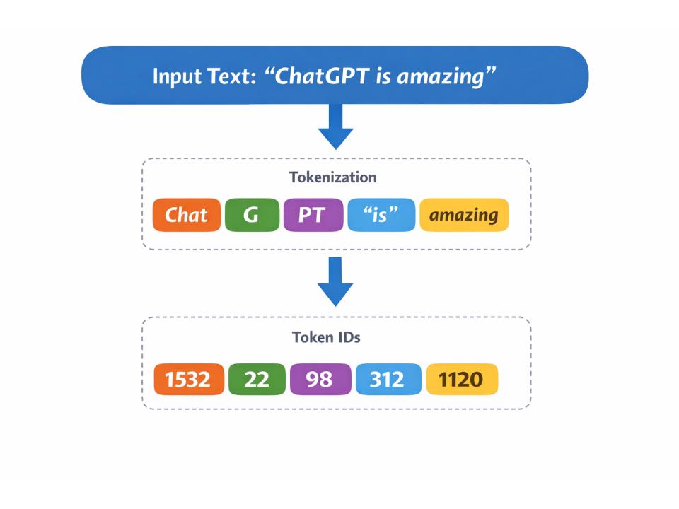
Tokenization breaks text into chunks (tokens) and maps each to an integer ID.
"Hello world"→["Hello", " world"]→[15496, 995]
Tokens aren’t always words. Common words might be single tokens; rare words get split:
"unhappiness"→["un", "happiness"]→ 2 tokens"the"→["the"]→ 1 token
Byte-Pair Encoding (BPE) is the standard algorithm. It starts with characters and iteratively merges the most frequent pairs until it hits a vocabulary size (typically 32k-100k tokens).
Why this matters to you:
- Billing is per token, not per word
- Context limits are in tokens (~1000 tokens ≈ 750 words)
- Rare words cost more tokens (bad for non-English languages, code, etc.)
3. Embeddings: Building the Input Matrix
Now we have token IDs like [15496, 995]. But these are just arbitrary integers - the model doesn’t know that 15496 means “Hello”.
We need to convert these IDs into vectors that capture meaning. This is where embeddings come in.
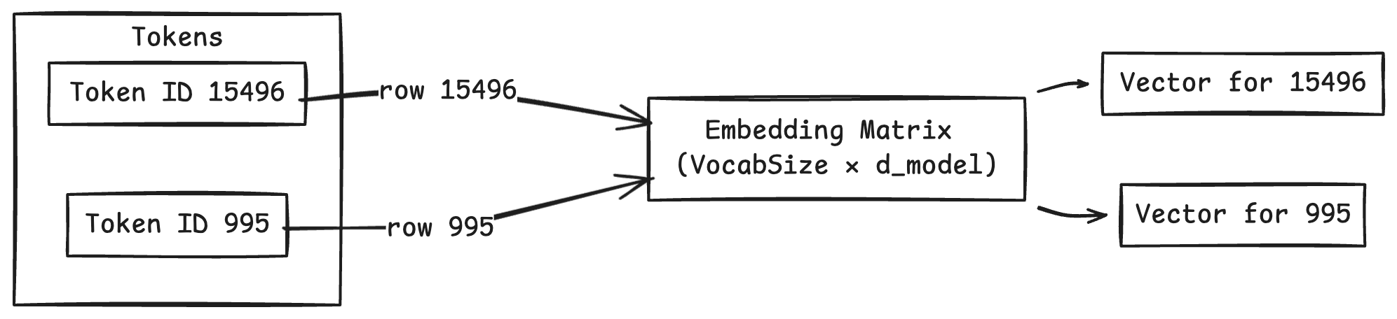
The Embedding Matrix
The model has a learned Embedding Matrix of shape [vocab_size, embedding_dim].
vocab_size: number of tokens in vocabulary (e.g., 50,000)embedding_dim: size of each embedding vector (e.g., 4096)
Each row of this matrix is the embedding for one token. To get an embedding, we simply look up the row for that token ID.
Token ID 15496 → look up row 15496 → [0.12, -0.34, 0.98, ...] (4096 numbers)
From Tokens to Input Matrix
If our input has 5 tokens, we look up 5 rows, giving us:
Input Matrix X: shape [5, 4096]
- Row 0: embedding for token 0
- Row 1: embedding for token 1
- ...
- Row 4: embedding for token 4
This input matrix X is what flows through the entire Transformer. Every subsequent operation transforms this matrix - changing its values but keeping its shape (roughly).
Why Embeddings Work
These embedding vectors are learned during training. The model adjusts them so that:
- Similar words have similar vectors
- Relationships are preserved geometrically
Famous example: King - Man + Woman ≈ Queen
This vector arithmetic works because the model learned that the direction from “Man” to “Woman” is similar to the direction from “King” to “Queen”. Meaning becomes geometry.
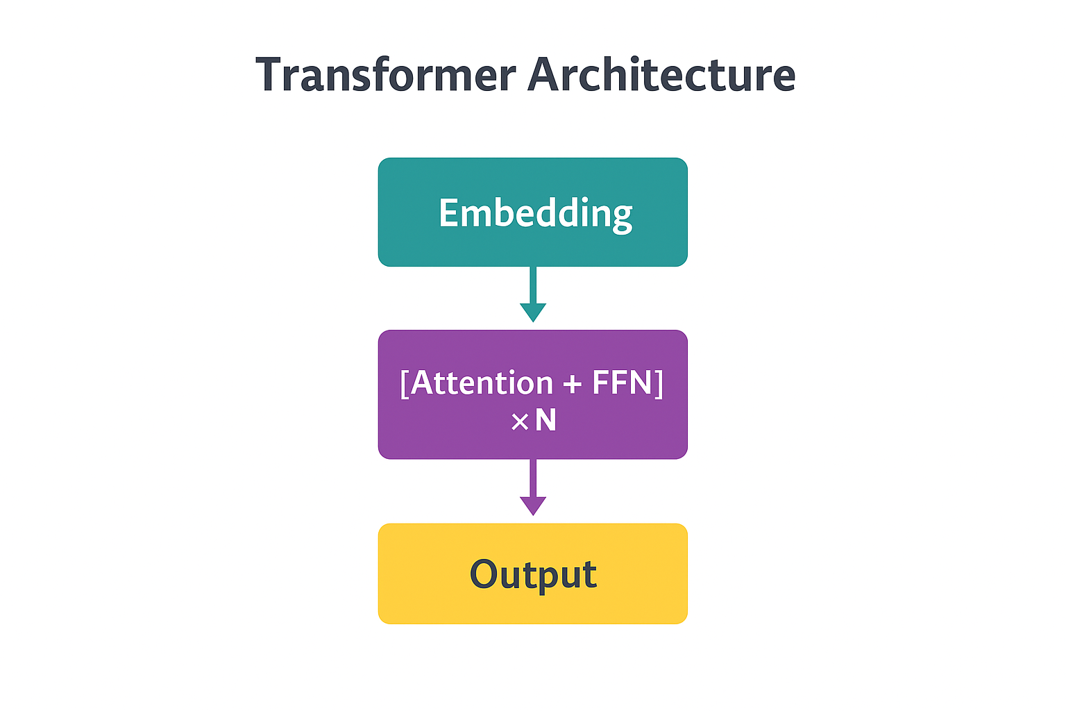
4. The Transformer: Transforming the Input Matrix
The Transformer architecture was introduced in the landmark 2017 paper “Attention Is All You Need” by Vaswani et al. It replaced previous sequence models (RNNs, LSTMs) with a purely attention-based architecture that could be parallelized efficiently on GPUs. Every modern LLM - GPT, Llama, Claude, Gemini - is built on this foundation.
Here’s the big picture of what happens inside an LLM:
Input Text
    ↓
[Tokenization] → Token IDs: [1532, 38, 2898, 318, 1049]
    ↓
[Embedding Lookup] → Input Matrix X: shape [5, 4096]
    ↓
[Transformer Layer 1] → Transformed Matrix: shape [5, 4096]
    ↓
[Transformer Layer 2] → Transformed Matrix: shape [5, 4096]
    ↓
... (repeat 96 times for GPT-3)
    ↓
[Final Layer Norm] → Output Matrix: shape [5, 4096]
    ↓
[Output Projection] → Logits: shape [5, 50000]
    ↓
[Softmax on last row] → Probabilities for next token
Each Transformer layer refines the representations. Early layers might capture syntax; later layers capture meaning, context, and reasoning.
Important: These Transformer layers ARE the “layers” of the neural network. When we say “GPT-3 has 96 layers,” we mean 96 Transformer layers stacked on top of each other.
Let’s break down what happens inside each Transformer layer.
4.1 Positional Encoding: Knowing Word Order
There’s a problem: nothing so far tells the model that “Dog bites man” and “Man bites dog” are different. The embedding for “Dog” is the same regardless of position.
Positional Encoding adds position information to each embedding. Before entering the Transformer, we modify our input matrix:
X = X + PositionalEncoding
The original Transformer used mathematical functions (sine and cosine waves at different frequencies). Modern LLMs often learn position embeddings directly or use techniques like Rotary Position Embeddings (RoPE).
Why this matters: Positional encoding is why models have context limits. The scheme must handle positions it saw during training.
4.2 Self-Attention: How Tokens Talk to Each Other
This is the heart of the Transformer. Self-attention lets each token “look at” all other tokens and gather relevant information.
The Intuition
Consider: “The cat sat on the mat because it was tired.”
What does “it” refer to? The cat. To understand “it”, the model needs to attend to “cat” - to pull information from that position into the current position.
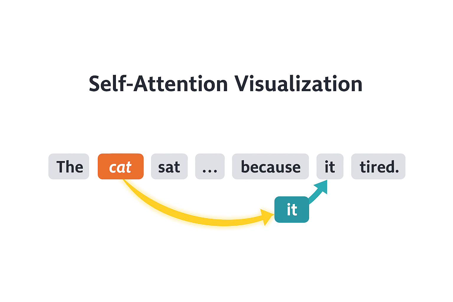
Self-attention computes, for every token, which other tokens it should pay attention to.
The Math: From Input to Output
Let’s trace exactly what happens. We start with our input matrix X with shape [seq_len, d_model] (e.g., [5, 4096]).
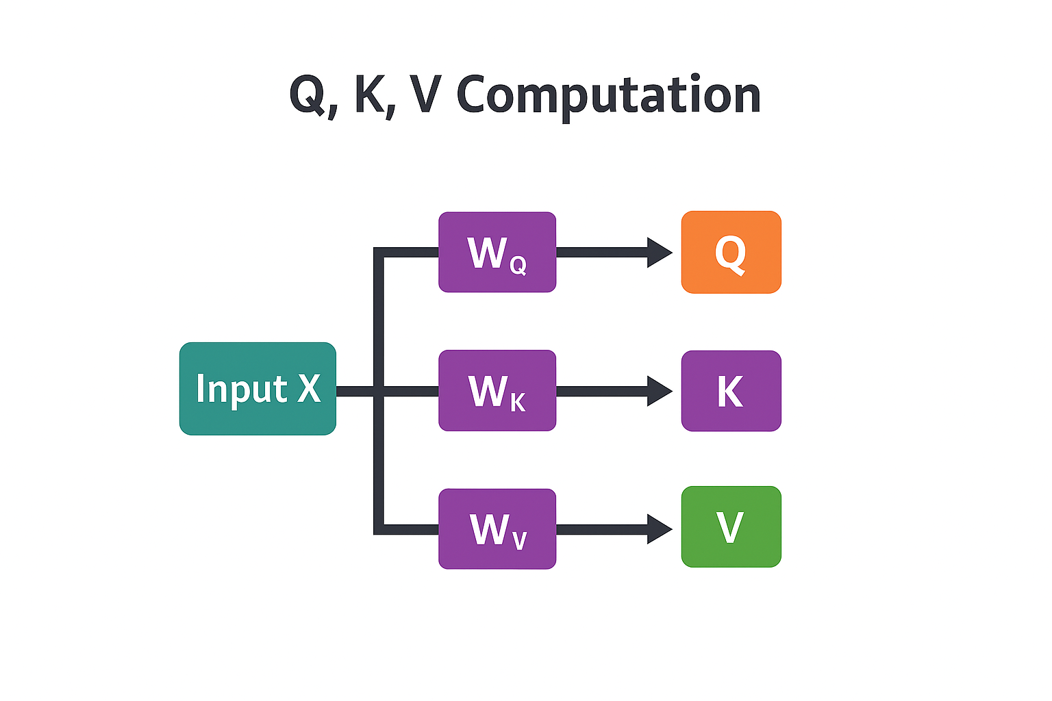
Step 1: Create Q, K, V matrices
We project X into three different representations using learned weight matrices:
Q = X × W_Q    (Query: what am I looking for?)
K = X × W_K    (Key: what do I contain?)
V = X × W_V    (Value: what information to pass along?)
Where:
W_Q,W_K,W_Vare learned weight matrices, each of shape[d_model, d_k]- Result: Q, K, V each have shape
[seq_len, d_k]
Think of it this way:
- Query for each token asks: “What information do I need?”
- Key for each token advertises: “Here’s what I have”
- Value for each token holds: “Here’s the actual information”
Step 2: Compute attention scores
How much should token i attend to token j? We measure similarity between token i’s Query and token j’s Key using dot product:
Attention Scores = Q × K^T
Where K^T means K transposed (rows become columns).
Result: a matrix of shape [seq_len, seq_len] where position (i, j) tells us how much token i should attend to token j.
Step 3: Scale the scores
The dot products can get very large, which causes problems for the next step. We scale down:
Scaled Scores = Attention Scores / √d_k
Dividing by √d_k (square root of the key dimension) keeps values in a reasonable range.
Step 4: Apply softmax
Convert scores to probabilities. For each row (each token), softmax makes the values sum to 1:
Attention Weights = softmax(Scaled Scores)
Now each row contains a probability distribution over all tokens - how much attention to pay to each.
Step 5: Weighted sum of values
Finally, use these attention weights to compute a weighted average of the Value vectors:
Attention Output = Attention Weights × V
Result: shape [seq_len, d_k] - a new representation where each token has gathered information from other tokens based on relevance.
The full formula:
Attention(Q, K, V) = softmax(Q × K^T / √d_k) × V
Masked Attention
For language models, we add one constraint: a token can’t see future tokens (that would be cheating - we’re trying to predict them!).
Masking sets attention scores for future positions to negative infinity before softmax. This makes those weights become 0 after softmax.
4.3 Multi-Head Attention: Multiple Perspectives
One attention mechanism can only focus on one type of relationship. But language is complex - we might need to track syntax, semantics, and coreference simultaneously.
Multi-Head Attention runs several attention operations in parallel, each with its own W_Q, W_K, W_V. Each “head” can learn to attend to different patterns:
- One head might track subject-verb relationships
- Another might focus on nearby words
- Another might handle coreference (like “it” referring to “cat”)
The outputs from all heads are concatenated and projected:
MultiHead = Concat(head_1, head_2, ..., head_h) × W_O
Typical LLMs use 32-128 heads.
4.4 Feed-Forward Network: Processing Each Position
After attention, each position passes through a Feed-Forward Network (FFN) - a simple two-layer neural network applied independently to each token:
FFN(x) = ReLU(x × W1 + b1) × W2 + b2
Where:
W1expands the dimension (e.g., 4096 → 16384)- ReLU is an activation function:
ReLU(x) = max(0, x) W2projects back down (16384 → 4096)
The FFN is often described as where the model stores “knowledge”. The expanded middle layer creates space for encoding facts and patterns.
Why do we need FFN? Attention alone isn’t enough:
- Attention = “gather” - it combines information from different positions (weighted averaging), but doesn’t really process that information
- FFN = “think” - it’s a non-linear transformation that processes the combined information
- Research shows factual knowledge (“Paris is the capital of France”) is encoded in FFN weights, not attention weights
- Without FFN, the model would just be mixing tokens without doing any real computation
4.5 Residual Connections & Layer Normalization
After each sub-layer (attention or FFN), we add the input back to the output:
output = LayerNorm(x + Sublayer(x))
Two things are happening here:
Residual Connection (x + Sublayer(x)): We add the original input to the output. This helps gradients flow during training - without it, gradients vanish as they propagate backward through 96 layers.
LayerNorm is a function (not just addition) that normalizes the values:
LayerNorm(x) = γ × (x - mean) / √(variance + ε) + β
It computes the mean and variance of x, normalizes to mean=0 and variance=1, then applies learnable scale (γ) and shift (β). This keeps activations in a reasonable range - without it, values would explode or vanish through many layers.
Putting It Together: One Transformer Layer
One Transformer layer does:
1. attention_out = MultiHeadAttention(X)
2. X = LayerNorm(X + attention_out)     ← residual connection
3. ffn_out = FFN(X)
4. X = LayerNorm(X + ffn_out)           ← residual connection
5. Return X
The input and output have the same shape. Stack 96 of these layers (for GPT-3) and you have an LLM.
What Gets Learned During Training (The Parameters)
When we say a model has “70 billion parameters,” we mean all the learnable weights across the entire network. For each Transformer layer, the model learns:
| Component | What’s Learned | Count per Layer |
|---|---|---|
| Attention | W_Q, W_K, W_V for each head | 3 × num_heads matrices |
| Attention | W_O (output projection) | 1 matrix |
| FFN | W1 (expand) and W2 (contract) | 2 large matrices |
| LayerNorm | γ (scale) and β (shift) | 2 vectors per norm |
Plus the Embedding Matrix (shared across the model) and sometimes the Output Projection.
Multiply by 96 layers and you get billions of parameters. All of these are randomly initialized, then adjusted through training to minimize prediction error.
5. Getting the Output: From Matrix to Words
After all Transformer layers, we have an output matrix of shape [seq_len, d_model]. How do we get the next word?
The Output Projection
We only care about the last position (that’s where we predict the next token). We take that row and multiply by an output projection matrix:
logits = output_row × W_vocab
Where W_vocab has shape [d_model, vocab_size] (e.g., [4096, 50000]).
Result: a vector of 50,000 numbers (one per possible token) - these are called logits.
Softmax: Logits to Probabilities
Apply softmax to convert logits to probabilities:
P(token_i) = exp(logit_i) / Σ exp(logit_j)
Now we have a probability distribution over all possible next tokens.
Choosing the Next Token
Several strategies:
Greedy: Pick the highest probability token. Deterministic but often repetitive.
Temperature: Scale logits before softmax. Higher temperature = flatter distribution = more randomness.
Top-K: Only consider the K most likely tokens, then sample.
Top-P (Nucleus): Include tokens until cumulative probability exceeds P (e.g., 0.9).
In practice, APIs use combinations of these.
Autoregressive Generation
LLMs generate one token at a time:
- Process prompt → get probability for next token
- Sample a token
- Append to input
- Repeat
This is autoregressive - each token depends on all previous tokens.
The KV Cache
Here’s an optimization insight: when generating token 10, we need attention with tokens 1-9. But tokens 1-9 haven’t changed! Why recompute their Keys and Values?
The KV Cache stores K and V for all previous tokens. For each new token, we only compute Q, K, V for that token, then reuse cached values.
Trade-off:
- Without cache: O(n²) compute per token
- With cache: O(n) compute per token
- Cost: Memory grows with sequence length
This is why long-context models need massive VRAM - they’re caching KV for the entire context.
6. Training: From Random to Intelligent
LLM training happens in phases.
Phase 1: Pre-training
Goal: Learn language patterns and world knowledge.
Data: Trillions of tokens - web scrapes, books, Wikipedia, GitHub.
Objective: Next-token prediction. Given tokens 1 to n, predict token n+1.
Result: A “base model” good at completing text but not following instructions. Ask “What is 2+2?” and it might respond “What is 3+3?” - continuing the pattern rather than answering.
Scale: This is expensive. GPT-4 scale pre-training costs tens of millions of dollars.
Phase 2: Supervised Fine-Tuning (SFT)
Goal: Teach instruction-following.
Data: Curated (prompt, response) pairs.
Process: Continue training on this data.
Result: An “Instruct” model that answers questions.
Phase 3: Alignment (RLHF / DPO)
Goal: Align with human preferences - helpful, harmless, honest.
RLHF:
- Generate multiple responses
- Humans rank them
- Train a reward model on rankings
- Use RL to optimize the LLM for high reward
DPO: Simpler alternative - optimize directly on preference pairs without a reward model.
7. Scaling Laws
Performance scales predictably with compute, data, and parameters.
Chinchilla Scaling Laws (2022):
- For fixed compute, there’s an optimal model size / data ratio
- Many early LLMs were “undertrained” - too big for their data
- Llama models follow this more closely
Emergent Abilities: Some capabilities only appear at scale - small models can’t do chain-of-thought reasoning. This makes capability prediction hard.
8. Practical Considerations
Quantization: Reduce precision (FP32 → FP16 → INT8 → INT4) to shrink models and speed up inference with minimal quality loss.
Distillation: Train a small “student” to mimic a large “teacher”. The student learns from soft probability distributions.
Context Length: Attention is O(n²). Techniques like sparse attention, sliding windows, and grouped-query attention (GQA) help manage this.
Summary
| Concept | What It Is | Why It Matters |
|---|---|---|
| Neural Network | Layers of matrix operations | The fundamental compute unit |
| Tokenization | Text → integer IDs | Determines cost and limits |
| Embeddings | IDs → Input Matrix | Meaning as geometry |
| Self-Attention | Q, K, V → weighted combination | Core reasoning mechanism |
| FFN | Two-layer network per position | Where knowledge is stored |
| Residual Connections | Add input to output | Makes deep networks trainable |
| KV Cache | Store K, V for past tokens | Makes generation fast |
| Pre-training → SFT → RLHF | Three-phase training | Random → smart → aligned |
This covers the core mechanics. There’s more to explore - mixture of experts, efficient attention variants, multimodal extensions - but if you understand what’s here, you can read the papers and follow along.
References & Further Reading
Videos
3Blue1Brown - “But what is a neural network?” - YouTube - The best visual introduction to neural networks.
3Blue1Brown - “Attention in transformers, visually explained” - YouTube - Beautiful visualization of how attention works.
Andrej Karpathy - “Let’s build GPT: from scratch, in code” - YouTube - 2-hour walkthrough building a GPT from scratch. Highly recommended.
Andrej Karpathy - “Intro to Large Language Models” - YouTube - 1-hour overview of what LLMs are and how they work.
StatQuest - “Transformer Neural Networks Clearly Explained” - YouTube - Clear, step-by-step explanation with visuals.
Articles & Blog Posts
Jay Alammar - “The Illustrated Transformer” - Blog - The go-to visual guide for understanding Transformers.
Lilian Weng - “The Transformer Family” - Blog - Comprehensive overview of Transformer variants.
Chip Huyen - “Building LLM applications for production” - Blog - Practical engineering considerations.
Sebastian Raschka - “Understanding Large Language Models” - Blog - In-depth technical breakdown.